How to manually calculate Tukey’s Honestly Significant Difference (HSD) for comparing factor levels

I was recently asked by a client to explain how the Tukey’s HSD (Honestly Significant Difference) is calculated, but I “honestly” didn’t know how it was done. So I did a little research, and wanted to share it with you.

What is Tukey’s HSD?

To explain it as simply as possible, when you run a statistical test on a categorical factor that comes up significant (p-value < 0.05), the interpretation is that at least one of the levels within that factor is different than at least one other level.

This is not a problem when there are two levels in a factor, such as Worker (Bill and Ted) or Shift (1st and 2nd) or Day Type (Weekday and Weekend).

However, when there are more than 2 levels, it can be confusing which levels are actually statistically different than the others, and sometimes they are all different from each other.

Here are some factors with more than 2 levels.

• Day of the Week (Mon, Tues, Wed, Thu and Fri)
• Worker (Bill, Ted, Abe and Joan)
• Supplier (Walmart, Target, Tesco)

Tukey HSD will look at each pair and determine which ones are actually different from each other.

If you’re familiar with a 2-sample t test, it will do something very similar, except it pools all the variation from all the levels, instead of the variation from only those two differences. You can read more about Tukey’s method for multiple comparisons on Minitab’s website or on Wikipedia under Tukey’s range test.

Performing the calculations by hand

Here is an excellent video showing how to hand calculate Tukey, so I don’t need to recreate this, but I will add some comments after you watch it.

Clarifications for the video

What is unclear in the video is how he comes up with 3.77 for the critical region values.

This value comes from a table called “Percentage Points of Studentized Range Distribution: q(t, v)” which is not a standard table you might run across. You can access a copy of the table here: https://web.stat.tamu.edu/~suhasini/teaching651/tables.pdf

With 3 different groups or treatment means (No Phone, Hand Held and Hands Free), and 12 error degrees of freedom (df, as shown in his ANOVA table), and alpha = 0.05, you can look up the critical value in that table.

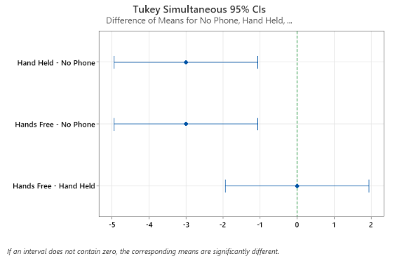
In his results, he showed that there were differences between “No Phone” and “Hand held” and “No Phone” and “Hands free”, but no difference between “Hand held” and “Hands free”.

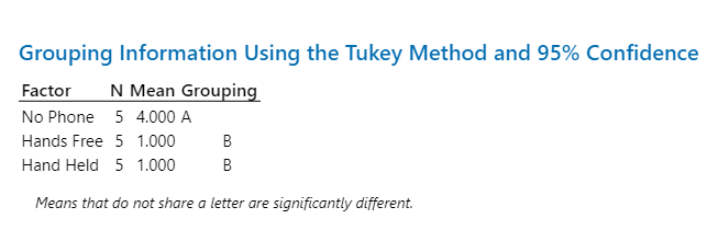
One of the reasons the Tukey test is popular is because it uses letters to make the summary simple to understand. If a level has the same letter as another level, then no difference between them. If they have different letters, then there is a statistical difference.

Factor       Groups
No phone     A
Hand held      B
Hands free     B

Performing Tukey HSD in Minitab

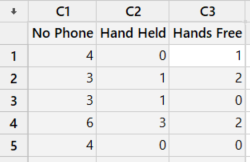
In Minitab, you can perform a Tukey test by taking the data set above, and running a One-Way Analysis of Variance (ANOVA).

Go to Stat > ANOVA > One-Way…

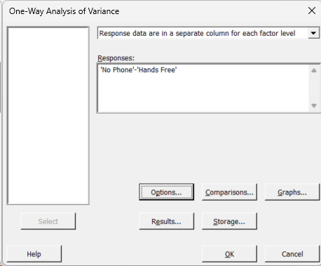
Click on the “Comparison…” button to select the tests you want to use (Tukey is one of the options).

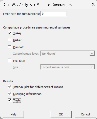
By default, the One-Way ANOVA test assumes equal variance.

However, if you go into the “Options…” button, and unselect “Assume equal variances” and then go back into the “Comparisons…” button, you will no longer be able to run a Tukey test, as it requires the equal variance assumption.

Instead, you will have the option to perform a Games-Howell test.

In Minitab, the results come out similar to what I created above, where “No Phone” has its own group (A), and “Hands Free” and “Hand Held” share a common letter (B), but both differ from “No Phone”

Minitab also outputs another data table, called the “Tukey Simultaneous Tests for Differences of Means” which shows the details of the grouping data above. The “Difference of Means” column looks at the means between each factor, which is pretty straightforward.

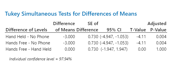
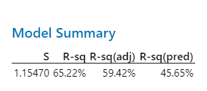
The “SE (standard error) of Difference” is a little more complicated to figure out. It is calculated by taking the S value from the ANOVA table, which is the square root of the mean square of error. In the video, he calculates the MS for Within (Error) as 1.333, so if you take the square root of that number, you get 1.1547.

Below, you can see the Minitab output for the ANOVA table with Adj MS for Error = 1.333 and S = 1.1547 as displayed in the Model Summary section.

The formula for SE for Difference is

S * square root (2/n)

Where n is the number of data points within each level of that factor. Since there are 15 data points, and 3 levels, then there are 5 data points within each level.

S = 1.1547
n = 5

SE Diff = 1.1547 * sqrt(2/5) = 1.1547 * sqrt(0.4) = 1.1547 * 0.632 = 0.73

Individual and Family Confidence Levels

One final consideration. Each comparison test will typically have an alpha of 0.05, which means there is a 5% chance of being wrong. If there are 3 comparisons being made (No Phone vs Hand Held, No Phone vs Hands Free and Hand Held vs Hands Free), and each one has a 5% chance of error, then there is a higher chance that at least one of these comparisons will results in an error. As you add more comparisons (more levels within the factor), this goes up even higher.

However, Tukey factors this into the analysis, but it also creates another potential issue.

If there are 10 comparison total, then Tukey test sets the alpha much lower for each individual test, in order to end up with an overall (family) error rate of only 5%. Each comparison is set at a smaller error rate of 0.65% (99.35% confidence). This prevents the higher risk of errors when concluding that levels are different (when they really are not), but instead it will make it harder to detect differences between each level when there is an actual difference, since you need a higher threshold in order to detect it compared to when it was set at 5%.

You can read more about this on Minitab’s website, under “Understanding individual and simultaneous confidence levels in multiple comparisons“

We also have an article that explains how the Tukey test adjusts the factor level means when handling covariates

Contact us if you have any questions about the Tukey test, as this topic is not covered in any Green Belt or Black Belt courses currently.